Visualise Data After Missing-Value Handling — visualize

Produces scatter plots of each numeric column vs row index (time order). At most 4 subplots are shown per page – if there are more than 4 numeric columns, multiple plots are printed sequentially. When imputation was performed, imputed points are highlighted in red.

Usage

visualize_data(
  handle_result,
  raw_data = NULL,
  cols_per_page = 4L,
  n_sample = 10L,
  verbose = TRUE,
  time_col = NULL,
  x_col = NULL,
  y_col = NULL
)

Arguments

handle_result: The list returned by handle_missing().
raw_data: data.frame. The original (pre-cleaning) dataset. Required when handle_result$action == "impute".
cols_per_page: Integer. Maximum subplots per page. Default 4.
n_sample: Integer. Rows to show in before/after console table. Default 10.
verbose: Logical (default TRUE).
time_col: Character. Name of the datetime column to use as x-axis. If NULL (default), row index is used instead.
x_col, y_col: Ignored. Kept for backward compatibility.

Value

An invisible list with elements scatter_plots (a list of ggplot objects, one per page) and before_after (data.frame or NULL).

Examples

data(airquality)
ana   <- missing_analysis(airquality, plot = FALSE, verbose = FALSE)
clean <- handle_missing(ana, verbose = FALSE)
viz   <- visualize_data(clean, raw_data = airquality)

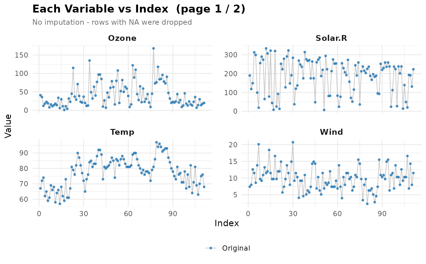#>   [Plot 1/2] columns: Ozone, Solar.R, Wind, Temp

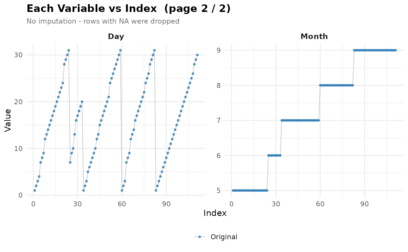#>   [Plot 2/2] columns: Month, Day
#>